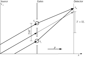
Can refer to slits in time as gates or chopper; slits most conventional.
Use x dimension as carrier, as signal.
Need both gate and particle to vary in time, therefore most appropriate to use kernel and Gaussian test function model.
Work in non-relativistic arena, using time/momentum representation.
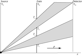
Break up by rays, making us automatically compliant with the requirement for geodesic time. For fixed initial momentum and endpoint, each ray is a geodesic.
The simplest initial wave function we could work with would be a direct product of a time and a momentum part:
However, as will be discussed below, this is a bit too simple.
Associate with each ray a correlated wave function in time:
With L the distance from the source to the gate, and is the time, treat laboratory time and momentum as related by the classical momentum/laboratory time relationship:
This is not a terribly sophisticated approximation; but it is simple.
Sum over all rays to get the final result.
Work primarily with Gaussian gates, rather than the more traditional square. Suggested by [Feynman-1965d]. Easier to work with and better fit to Lindner's experiments. As by Morlet wavelet decomposition, any gate may be written as sum over Gaussians, is in a certain sense fully general.
Outline
Start by looking at the free case.
Wave function in , non-relativistic:
Wave function in p :
Assume starting at position zero:
Carrier in momentum space
Standard quantum theory given by carrier part alone.
Probability density:
Using obvious definition:
Carrier in laboratory time
Actual measurements are of clicks per unit time, not of momentum. Translate using classical momentum/laboratory time relationship. Average:
in laboratory time as a function of :
And as a function of :
Wave function as a function of (keeping only quadratic and lower terms in ):
Expanded:
Or:
Dispersion in laboratory time:
Kinetic energy as laboratory energy:
Probability density:
Direct product wave function in quantum time
Now add in quantum time.
First try a direct product initial wave function:
With the quantum energy the average quantum energy for the beam:
And initial expectation of quantum time:
At this point we do not know the dispersion in time. We may estimate it from the dispersion in momentum using the method in Estimates of uncertainty in time/energy:
Another approach is to use an earlier gate to prepare the wave function, thus forcing the issue. But we have to solve the one gate problem before we can do that. For now, we will posit it as estimated "somehow".
Expression for relative time wave function at detector:
Get:
With definitions:
And:
Probability density in time:
Full probability density:
To get distribution in time, integrate over distribution in momentum:
Because time and momentum parts uncorrelated, total dispersion in time is dispersion of quantum time part:
There is no effect on the dispersion in time of the dispersion in momentum. This is unphysical.
Correlated wave function in quantum time
We therefore look at an initial wave function with time and momentum linked. Associate a wave function in time with each ray, then add together at the end.
More natural. In energy momentum space, would naturally assume energy part of wave function corresponding to each ray centered on that ray, not on the average. Taking the inverse Fourier transform to get the wave function in time, we get time wave function centered on each ray.
Do as above, but unbar our wave functions and our kernels.
First, define relative time on a per momentum basis:
Wave function, in relative time:
Energy now a function of specific momentum:
Again, average quantum time at start zero, analysis non-relativistic.
With:
Probability density in time for a specific ray:
Full probability density:
Normalized correctly:
Each wave function in time centered on a different p and therefore different . To combine expand laboratory time as a function of ray:
Probability density (again keeping only up through quadratic order in expansion):
Trace out the momenta:
Define dispersion associated with quantum time:
To get probability density in time alone:
Gives:
With dispersion:
Define angle in laboratory time by:
This is a proxy for energy: the greater the dispersion in energy, the greater in angle.
Full dispersion in time is dispersion associated with quantum time plus dispersion associated with momentum:
With angular dispersion:
So angular part of dispersion comes equally from quantum time and from standard quantum theory parts.
Since we can make gate as short as we like, in principle, can make angular dispersion as great as we like.
Reduction to standard quantum theory
Representation of function:
Apply:
Get:
So:
Gives:
If we assume dispersion in time narrow but not zero, can simplify by expanding distribution in p in powers of . However as we have limited functions to Gaussians, no need here.
Shape of Gaussian gate
In laboratory time:
In quantum time:
Standard quantum theory
Expression for final wave function:
Gate:
Or:
With definitions:
The further from the source the gate is, the greater is, and the narrower the effective width of the gate, relative to the spread in the beam.
The integral is trivial. Wave function is:
Look at case of beam centered on gate:
Probability density:
Effective dispersion:
Width dominated by the narrower of the beam and gate, whichever that is.
In laboratory time get:
We can rewrite the dispersion coefficient as:
From this it is obvious that the effect of the gate is always to reduce the dispersion. Unless the gate is much wider than the particle, it will clip the edges of the particle, narrowing it.
Temporal quantization
As noted, use the time/momentum representation. Particularly simple separation of standard quantum theory and temporal quantization parts into the momentum and time parts. Dependence of time part on laboratory time goes as mass, nice fit to dependence in kernel.
Expression for final wave function:
First look at case of beam centered on gate:
Integral now a variation on the usual free integral:
Assume beam has not widened in quantum time appreciably in trip from source to gate:
The dispersion in quantum time therefore one half the harmonic mean of the gate and initial dispersions:
As we would expect, a narrow gate (narrow in time) will reduce the dispersion in time: and therefore increase the dispersion in quantum energy.
Final wave function:
Probability density in quantum time:
With parallel definition:
Probability density in momentum unchanged.
Integrate over p to get total probability density:
Result:
With definition:
Spelled out:
Effective dispersions:
Similar to the results for the free case, except have substituted effective for free dispersions, due to the gate.
In temporal quantization have a constant term for the dispersion and a linear term. Linear corresponds to the angular dispersion.
Standard quantum theory result similarly spelled out:
In standard quantum theory, we have only the linear term. The behavior with respect to very different: as gets smaller, the dispersion gets smaller as well. No diffraction; time a parameter.
In temporal quantization, we can make the angular dispersion as large as we like by decreasing , as we would expect from the uncertainty principle.
Beam off-axis
Now look at case when beam comes in off-axis:
With definition:
Rewrite:
Use narrow beam approximation as before.
Effective dispersion is same as in the on-axis case.
With normalization constant:
And effective offset in as:
Note that normalization constant always less than one unless we are on-axis, in which case it is one. Being off-axis reduces overall size.
Same sense as offset for gate:
Effect is as if it started a bit earlier or later in time.
Pulling the whole wave function together:
Or:
Recalling:
This reduces, as it should, to on-axis result when:
In energy momentum space:
So energy part centered on each separate ray in momentum space, analogous to behavior in time and momentum. Note that the laboratory energy now includes a quantum energy part:
Further, dispersion in energy inverse of dispersion in time:
So for small gates: arbitrarily large dispersion in quantum energy.
Takeaway: by making the gate short, and waiting a bit, make the dispersion in time as large as we wish. No longer dependent on estimates of ; can force the issue.
Can use as experiment in own right or as preparatory stage for others.
Will assume this in following.
Wave function as sum over the single slit wave functions:
Look at probability density:
Particularly at interference terms:
Impact possible in two areas:
-
Spacing of fringes.
-
Dispersion at each fringe.
As we will see below, usual graphic analysis does not work well.
Need more explicit criteria.
In simple cases we look at, can still locate fringes by inspection.
More generally, we can work out the location of the fringes with respect to time by looking at the derivatives of the probability density with respect to time. Crests given by points when:
With width at crests then given by:
For comparison, look at hard-edged case.
Two slits in a row in :
Two slits in a row in p :
With P 's:
In the ray model we are using, there is no interference. The "fast" rays come out the first slit, the "slow" rays come out the second, they do not meet.
This is expected from "time is a parameter".
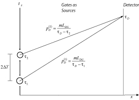
In the Lindner experiment below, the two gates are both equally sources of fast and slow particles, there is no such limit.
If we are using Gaussians same result for same reason, with minor complication that there could be some overlap from the Gaussian tails.
In temporal quantization, have:
But now diffraction from gates is possible.
Now, treat gates as separate but correlated sources. Closer to Lindner.
Will treat in fact as free particle sources; reuse results from Free case, with a bit more care as to starting points.
Plane waves
Amusing note: with plane waves, no interference in time. If the wave has a momentum , then the first part will have an initial phase of, say, , and accumulate a further phase proportional to the time to the detector:
Second:
Difference:
The difference is not a function of , so there is no interference pattern at the detector.
Gaussian test functions
Initial wave function:
Start at zero:
Wave function at detector:
Consolidate initial phase:
Convert to laboratory time using classical momentum/laboratory time relationship:
With definitions:
And:
Without loss of generality, center the gates in time and phase:
Gives:
Now:
Pull out the common factor:
Full wave function:
Probability density is:
At longer times, larger distances:
Probability density goes to:
In terms of angles (constant with ):
Period is:
As a quick check, if gates are not separate, wave function at detector is multiplied by four:
Now each ray has built in fuzziness in time.
Wave function
Work with the temporal quantization wave function from above. Wave function:
With:
As above, gives the difference in phase between the two gates.
As above, without loss of generality take:
Time:
Space:
As above, consolidate the phase differences into the :
At detector:
Time wave function:
Average location in time:
Momentum wave function:
Use narrow beam approximation:
Put parts together:
Rewrite using classical momentum/laboratory time relationship:
Now wave function is in terms of quantum time and momentum; no dependence on laboratory time.
Recall:
Common factor:
Interfering factor:
Probability density
Probability density is:
As with standard quantum theory, time part divides naturally into non-oscillatory and oscillatory parts:
Similar to corresponding expression for standard quantum theory, except that is a function of momentum.
Momentum part:
Probability density in time:
Expanded:
Non-oscillatory part already done, is two free functions offset from average by plus and minus :
Break out cosine as sum of exponentials:
The integral over p can be done but is uninstructively complex. Argue that we can drop quadratic oscillating term:
Get:
Define:
In long time limit:
Periodicity same as with standard quantum theory:
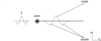
In Lindner et al's experiment, [Lindner-2005], strong short electric pulse ionizes electron. Like a dog shaking off water, can come off to right or left.
Photon in x , electric field in y , say. Shortest possible pulse (average field zero) can have two humps on left, one on right (or vice versa). Intense electric field can ionize electron, forcing to one side or other. If kicked by single pulse side, single gate diffraction. If kicked by double pulse side, double gate diffraction.
Impressive character of these experiments.
[Horwitz-2005]: Good analysis of time, there are subtleties to this.
Have dispersion from the original photon; spread in bound state in time may act as additional source of dispersion in time. Can estimate that as above.
See as a way to carry the bound electron's dispersion in quantum time/quantum energy out to where it can be seen. Provides a direct measurement of width of bound state in time.
Electric field
Assume photon going from left to right in x direction, centered at time zero on the atom at position zero. Look at polarization in the y plane.
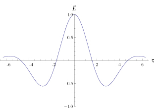
Photon wave vector in x , write electric field in y , as a Gaussian (using Greek letter for the electric field):
Have to subtract out the DC component. Corresponding Morlet wavelet already has the DC component subtracted out (by construction), so rewrite as:
It is more blessed to ask forgiveness than permission.
Looking for a simplified model that captures heart of the problem, making clear the differences between standard quantum theory and temporal quantization models.
Ionization only happens at peak of the field, so to some approximation, can represent as one kick or two.
Start off with a bound state. Represent the part that is kicked off as a Gaussian test function in momentum, centered on the kick momentum.
Represent the interaction itself as a Gaussian rather than a slit. Easier to deal with and actually more realistic, particularly when as note above an arbitrary gate can be built up – via Morlet analysis – from a set of Gaussian gates.
Ignore off-axis part of momentum; ignore and components of momentum.
Perturbation series
Generic series for kernel:
Only first term here. No interference with zeroth term because off to one side.
Explicit for standard quantum theory:
Explicit for temporal quantization:
Transition matrix
Standard quantum theory transition matrix has form:
Temporal quantization transition matrix, most obvious is a function in quantum energy.
For quantum energy of incoming photon, use its average, standard quantum theory energy.
These are guesses, but the simplest possible. For full realism, should go to quantum electrodynamics. But how to get to quantum electrodynamics without first working out reasonable expectations at the single particle level?
All together:
All dependence of matrix element on from electric field. For "single gate" case, standard quantum theory:
For "double gate" case, standard quantum theory:
As noted, can write an arbitrary gate as a sum over these, using Morlet wavelet decomposition.
If think of cosine as sum of two exponentials, only the term with positive frequency will contribute. Take x , the position of the atom, as zero. Look only at y component of electric field. Define function:
Single gate:
Double gate:
To include both cases use generic:
We treat the electric field as a classical force.
Initial wave function
Bound standard quantum theory:
In momentum space:
Evolution in time:
Where is the usual bound state energy.
Considered using direct product wave function here. However, open to same objections as in the free case. Therefore, using relative time, as above:
With:
As do not see the bound state as diverging along different rays, use the one wave function in quantum time.
Standard quantum theory
First two factors on the right, K , are the bound state wave function as it evolves in time:
Result:
Look at a crude example, in standard quantum theory:
Free wave function:
Therefore matrix element:
Write matrix element as product of function of p and :
Or for double gate:
Factoring of p and is welcome, but not essential.
Take the bound wave function in p as real. Approximate the term in p as a Gaussian:
With obvious definitions:
Result:
Since kernel in momentum is a function:
Can see as being average target for specified p . Change variables from p to :
Giving:
Expand function in powers of difference of time from average time:
Giving:
Temporal quantization
Go back to expression for series:
Using up various functions:
Expanding kernel and wave function in quantum time:
With:
Integral over is familiar one, pushing the free wave function along the trajectory from to :
Use approximation:
Get as result the correlated product of time and space parts:
Probability density:
To get probability density over time:
Or:
Standard quantum theory
Explicit expression:
Integrated:
Dominated by the case when the laboratory energy is conserved:
Ignore the variations in energy of particle depending on which part of the gate it came from; will assume below that when the particles comes from one of two different gates can no longer do this.
Here have:
As we pull detector back from source:
So see wave function go as:
Probability density:
Same as free case above, modulo the overall normalization. For simplicity write:
With normalization:
Temporal quantization
Initial dispersion in quantum time from initial dispersion in quantum energy:
The quantum time wave function is the free quantum time wave function, pushed out along the ray:
Therefore the time part of the probability density is the free time probability density from above:
Full probability density is:
Integral over :
Result:
Or:
Therefore result in case of a single gate is an increase in dispersion:
With estimate from bound states, of order:
Double source as sum of single source
Imaginary part is what is real here, looking for interference between gates.
Standard quantum theory
Analysis and results essentially same as before.
Wave function as sum of single wave functions:
Or:
Energy:
Assume envelope slowly varying:
Keep linear variation with laboratory time, so probability density goes roughly as:
Temporal quantization
As above, the free particle wave function in time moves along the ray from each gate. The only difference is that the phase difference between is created by the bound state:
And the initial dispersion in time given by the dispersion of the bound state:
Giving the same result:
Model here simplified, to demonstrate principle.
Assumption of correlated state necessary but can only be justified from full analysis, i.e. at quantum electrodynamics level.
With that assumption, the experiment acts like an escalator, lifting the fuzziness in the atom out to the detector.
As orbit times can be order of 150 attoseconds, and current resolutions go down to 100 attoseconds, this would appear to be detectible in principle.