It is the outstanding feature of the path integral that the classical action of the system has appeared in a quantum mechanical expression, and it is this feature that is considered central to any extension of the path integral formalism.
Semi-classical approximation for path integrals gives a clear connection to classical picture: classical solutions found in the center of a quantum valley. References: [Feynman-1965d], [Schulman-1981], [Khandekar-1993], [Kleinert-2004], [Zinn-2005].
Semi-classical approximation is exact if the Lagrangian is quadratic or simpler. Lagrangian in temporal quantization more complicated; still we have exact solutions for the cases: Free propagator, Constant potentials, Constant electric field
Further, semi-classical approximation works well with wavelets.
We work with block time here.
In semi-classical approximation, rewrite path integrals in terms of fluctuations around the classical path. Path integral:
With:
The x's are four vectors.
Set variation with respect to to zero to get:
This gives classical equations of motion:
Rewrite coordinates as classical part plus variation:
First approximation for kernel
Full expression
With:
This is exact. It can be solved explicitly for quadratic part. Write kernel as:
With:
We can take over existing calculations with slight change in meaning, no change in wording. As we need proof for N dimensions, cite Khandekar, Kleinert, Zinn.
Differences between standard quantum theory and temporal quantization:
-
We go from three to four dimensions.
-
We rely on Morlet wavelets, not factors of or Wick rotation, for convergence. This is off-stage in any case.
-
In temporal quantization we have an indefinite mass matrix.
None of these differences are critical.
Result:
After the determinant hits its first zero, have to replace determinant by its absolute value and add a phase factor:
Where ν is a count of the number of zeros the determinant has gone through.
Free propagator
Calculation of free propagator using semi-classical approximation provides a useful check.
Lagrangian:
Euler-Lagrange equations:
Classical trajectory:
Lagrangian on classical trajectory:
Action:
Determinant of action:
Kernel:
In agreement with above.
Good for analysis of piecewise constant potentials, as for Aharonov-Bohm.
Lagrangian:
Change in action:
Change in kernel:
Electric and vector potentials are constants:
Change to kernel (from free case) is essentially a gauge change with the choice of gauge:
This has no more impact on probabilities than a gauge change would have.
However if the potentials are only piecewise constant, then we may see interference between paths. See Aharonov-Bohm experiments below.
Case of constant electric field.
Formally similar to that of the constant magnetic field, under interchange of x and :
Drop the mass over two term for this analysis, to play up the simililarities. Legitimate since it is a constant in any case.
Treatment here modeled on the one in Kleinert.
Derivation of kernel
In case of constant magnetic field in z direction, we would focus on x and y dimensions. Here we focus on and x .
Field:
Choose four potential to be in Lorentz gauge and also symmetric between and x :
Lagrangian:
Euler-Lagrange equations:
With definition:
Action for x and :
Integration by parts:
Use the equations of motion to show integral is zero.
Final form for action:
Euler-Lagrange equations:
Solutions:
Constants of integration inferred from the equations of motion:
Parts of action:
Action:
First term is square of Minkowski distance times a coefficient. Second term is a gauge term.
Determinant:
Kernel:
Meaning of gauge
Shifts of starting position show as gauge changes
Change in action:
Again, second term can be treated as a gauge term:
Gauge function:
See here need for laboratory time potential per above.
Comparison to magnetic kernel
Magnetic field in z direction:
Magnetic Lagrangian is:
Equations:
Action:
Magnetic kernel is:
Switch:
To get the same.
Verification
With choice of gauge above, Schrödinger equation is:
So Hamiltonian is:
When >0, kernel satisfies:
Which we may verify by direct calculation.
When goes to zero, we require:
For short laboratory times, we have:
Which is only a gauge transformation away from the kernel we just derived.
From the point of view of the semi-classical approximation, the principle effect of temporal quantization is to add fuzziness in time, a kind of Zeitbewegung from the German for time and motion by analogy to Zitterbewegung.
If we look at the particle in terms of paths, most paths will cross any particular boundary, i.e. a gate, many times, like a nervous cat.
We would like to understand why if temporal quantization is correct, we normally get good results when we break up a problem into zones and solve zone by zone, pasting the kernels together at the end. Shouldn't we have to explicitly include the paths that go back and forth across the zone boundaries?
If the Lagrangian is quadratic in small deviations from the classical path, then the semi-classical approximation is exact, so includes the effects of Zeitbewegung. We can use this to study the zone crossing question.
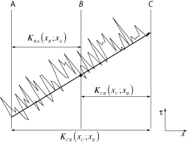
Consider a particle going from A to B to C. Assume that the semi-classical approximation is a "sufficiently good" approximation to the kernel from A to C. What are the effects of replacing this with the approximation where we use the semi-classical approximation to go from A to B, and then B to C, provided we choose B optimally? How good is:
The full action is sum of the two halves:
With one additional variation, of the coordinates at the interface:
If we choose for the coordinates of the crossing point the values that extremize the total action we will have recovered the full semi-classical approximation from the two halves.
Locate the crossing point by the variational method:
Note that the derivatives of the action with respect to the coordinates give the classical energy and momentum [Greenwood-1997]:
Therefore the required variational condition is equivalent to matching energy and momentum at the boundary:
And therefore matching up the kernels at the boundary by requiring conservation of energy momentum is exactly equivalent to computing the full semi-classical approximation from A to C.
And therefore, at least in the cases where the semi-classical approximation is a good approximation, we do not need to worry about multiple crossings of a boundary, provided we select the crossing point to preserve energy momentum conservation,
Refer to this as the Fresnel approximation; where we only paths that cross a gate once.
As an example, consider free case.
Free action:
Condition at boundary:
These are just energy momentum conservation at the boundary.
Semi-classical approximation gives a clear picture, as usual, of relationship between classical and quantum fields; the classical trajectory defines the location of a valley at the center of the quantum hills.
This helps to explains why temporal quantization not seen: expectation of obeys classical equation; unless we are explicitly probing dispersion in quantum time, we are unlikely to see any effects.
The analogy between kernels for constant electric and constant magnetic fields useful in finding an analog to the Aharonov-Bohm experiment.